Bifurcations

In this post I will discuss bifurcation.

“In general, a small variation in some parameter produces small, continuous changes in the system output, so that the system is said to be structurally stable. However, for some specific parameter values, a small variation can induce a strong qualitivative change in the solution. Such a behavior is called a bifurcation, and the system is said to be structurally unstable for these parameter values.”[1]

Consider the ordinary differential equation:

x_t  = r x - x^3

where r is the parameter of interest, subscript t is the time derivative of x. An equilibrium of the system is a point where the system remains unchanged or equivalently

x_t = 0

In our case if r is greater than zero then there are three equilibriums:

x = 0, -root(r), + root(r)

We can plot the derivative x_t against x:

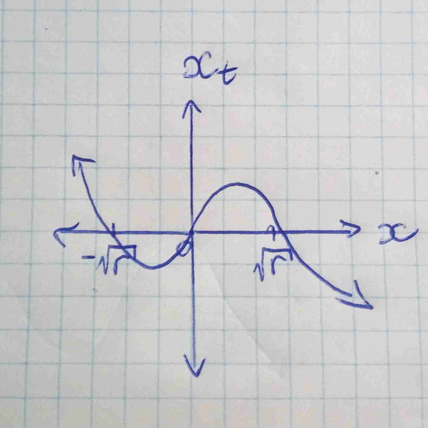
The first equilibrium is unstable since a slight perturbation will cause to move away from it (similar to a ball on top of a hill being slightly pushed will roll away). It is unstable because if x is slightly less than zero then the negative derivative (refer to previous plot) will cause x to decrease away from 0 and similarly if x is slightly greater than zero then the positive derivative will cause x to increase away from 0. Using similar logic the other two equilbiriums can be shown to be stable (a ball in a valley pushed will roll back).

When r is less than or equal to zero there is only one equilibrium (x=0 which is stable). Once again we plot x_t against x:

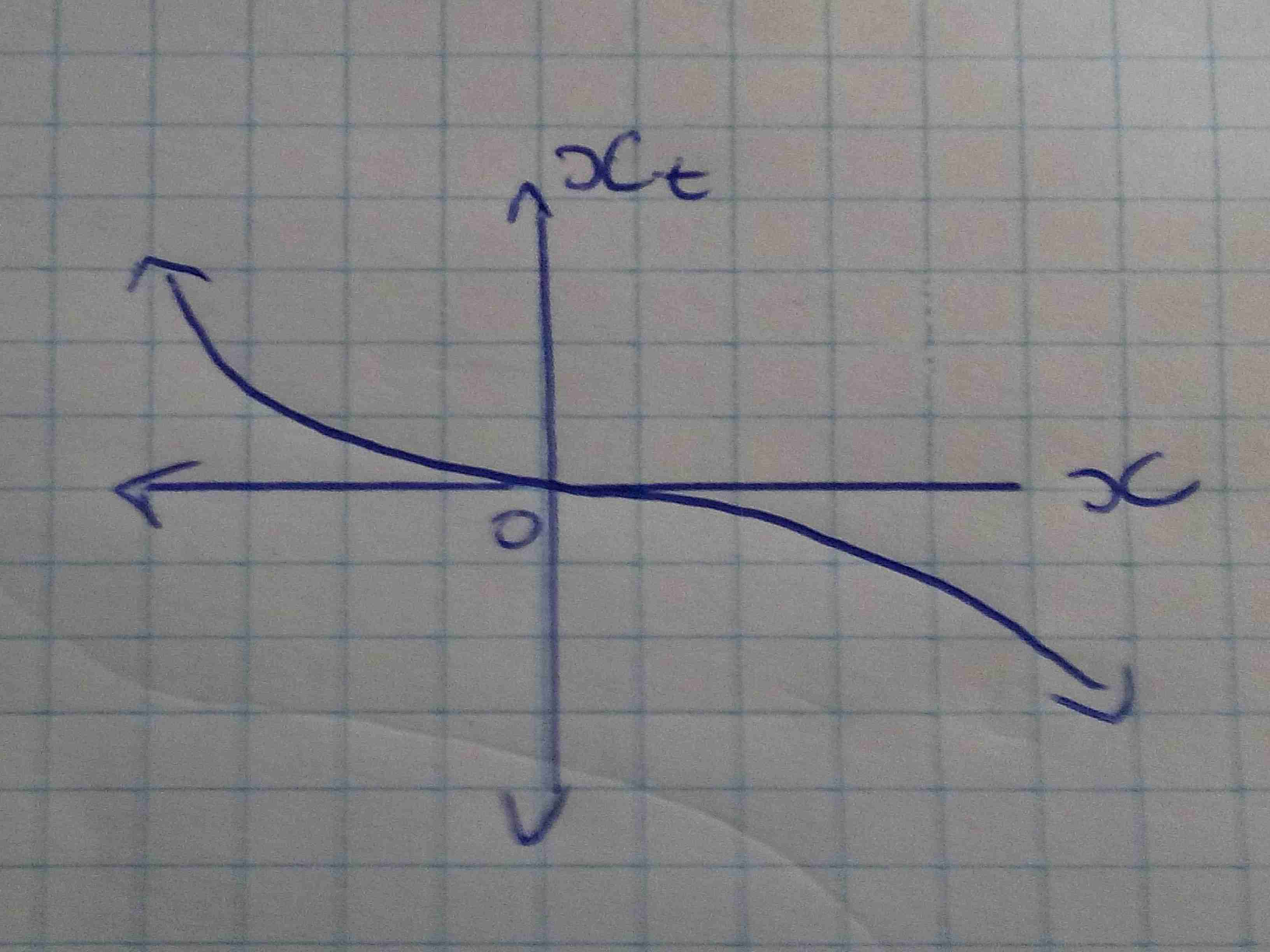
When varying r from negative to positive we move from one stable point to two stable points. r=0 is the bifurcation point where small variation will cause strong qualititative change in the solution.

Now let’s consider a more interesting system - the logistic map equation:

x_{t+1} = r x_{t} (1-x_{t})

where r is the parameter. We will restrict r to be in the range 0 to 4 (this provides that if x_{n} is between 0 and 1 then x_{n+1} will also be between 0 and 1 - can be checked via derivative tests). The logistic map reprents a population model where x_{n} between 0 and 1 represents the percentage out of a total maximum possible population. Below are some sample populations for different r values

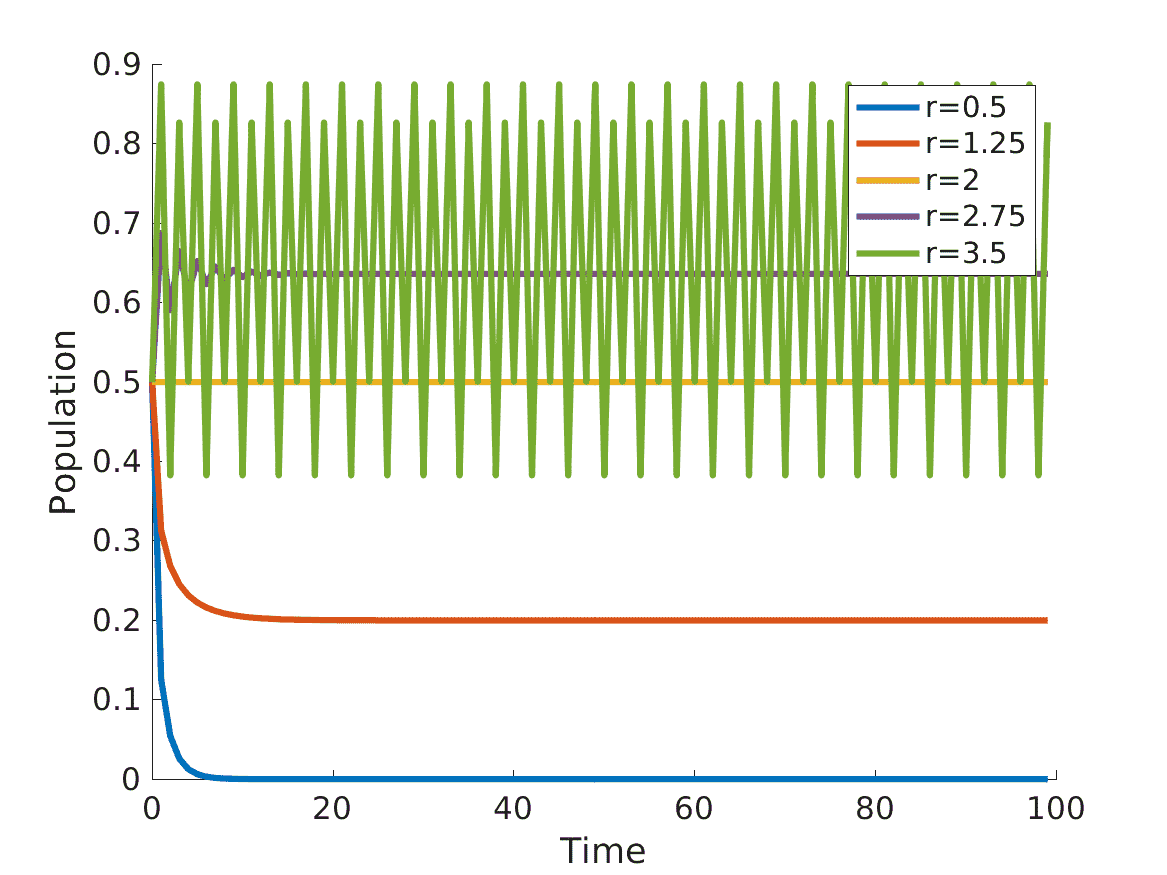
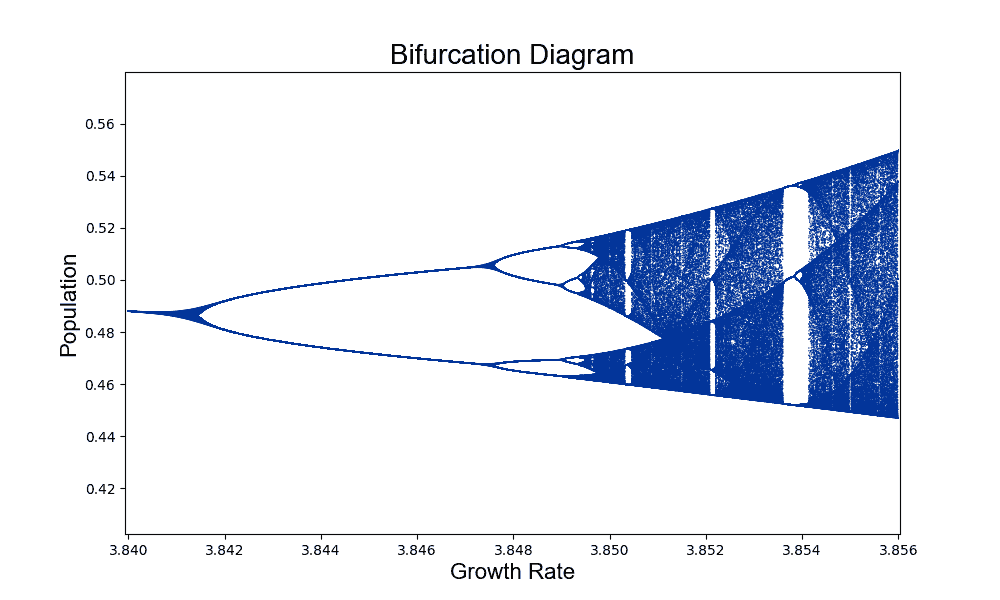
For r=0.5 the steady value is 0 meaning that the population starting at x_{0} = 0.5 will lead to population extinction (x_{n} = 0). For r=1.25 the population reaches steady state of about 0.2. r=2.75 and r=2 also reach a single steady state. Now for r=3.5 things get interesting - there are now 4 steady values about which the curve oscillates about regularly: 0.8269, 0.5009, 0.8750, 0.3828. By changing the parameter r from 2.75 to 3.5 we have change the amount of steady values from 1 to 4. This leads us to plot a bifurcation diagram. Below the diagram plots for various r (Growth Rate) the steady values. For r less than 3 there is only one steady value and at about 3 (bifurcation point) we now have two steady points and once r is about 3.5 there are four (as demonstrated earlier).

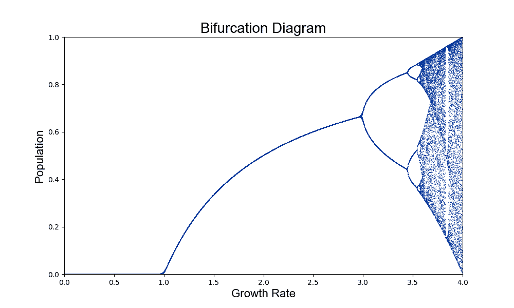
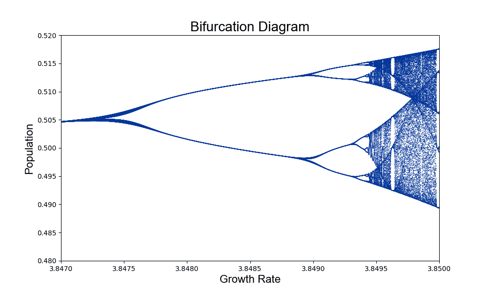
If we zoom in to a smaller range we see the following:

and if we zoom in even further we start noticing a fractal type pattern emerging - same structure at every scale. From the simple logistic map equation we obtain a beautiful pattern.

Some of the code used to generate the figures, insipiration as well as additional reading material can be found here:

Boccaletti, Stefano, et al. Synchronization: From Coupled Systems to Complex Networks. Cambridge University Press, 2018
Boeing, Geoff. “Visual analysis of nonlinear dynamical systems: chaos, fractals, self-similarity and the limits of prediction.” Systems 4.4 (2016): 37.
https://www.math.ucdavis.edu/~hunter/m207/m207.pdf
https://github.com/gboeing/pynamical