Stan working with Stan
Stan is a language used for statistical inference. Here we will investigate estimating the unknown length of a pendulum based on measurements of velocity and angle $\theta$. Two good examples to get started with Stan are
Here Stan will be used to estimate parameters - specifically the length of pendulum. Consider the pendulum equation
$ \frac{d^2 \theta}{d t^2} + \frac{g}{l} \sin(\theta) = 0$,
where $\theta$ is the angle of the pendulum, $g$ gravitational constant, $l$ is the pendulum length and $t$ is time. With damping added, the equation is now
$ \frac{d^2 \theta}{d t^2} + \frac{g}{l} \sin(\theta) + s \frac{d \theta}{d t} = 0$,
where $s$ is a damping constant.
Letting $v = \frac{d \theta}{dt}$, we get the following system of differential equations:
$\frac{d v}{dt} = - \frac{g}{l} \sin(\theta) - s v$
$\frac{d \theta}{dt} = v$.
We can encode the DEs in Stan as follows:
functions {
	real[] dz_dt(real t, real[] z, real[] params, real[] x_r, int[] x_i){
		real velocity = z[1];
		real theta = z[2];
		real g = 9.81;
		real damping = 5e-1;
		real length = params[1];

		real dv_dt = -(g/length)*sin(theta) - damping*velocity;
		real dtheta_th = velocity;

		return {dv_dt, dtheta_th};
	}
}
where dz_dt returns
$ \begin{bmatrix} \frac{d v}{dt} \\ \frac{d\theta}{dt}\end{bmatrix} $
evaluated at a particular $\theta$ and $v$. x_r and x_i are unused arguments that could be used to provide additional arguments to the function. The ODE is solved in
transformed parameters{
	real z[N,2] = integrate_ode_rk45(dz_dt, z_init, 0, ts, params, rep_array(0.0,0), rep_array(0,0), 1e-6, 1e-5, 1e6);
}
where the arguments to the ode solvers are provided by the data block:
data {
	int <lower = 0 > N;		//number of measurements
	real ts[N];			//the times at which measurements are taken
	real y_init[2];			//initial measured
	real y[N,2];			//measured velocity and theta
	real <lower = 0> sigma[2];	//sensor noise measurement standard deviation of velocity and theta
}
$N$ in this case is the total measurement counts where the $i^{\text{th}}$ measurement is taken at time ts[i]. The measurements along with an initial guess known as the prior will be used to estimate the length. The assumed initial conditions provided in y_init and y are the measurements of $v$ and $\theta$. In transformed parameters the first two arguments of rep_array(0.0,0), rep_array(0,0), 1e-6, 1e-5, 1e6 are NULL equivalent while the rest are ode solver specific. The user provided data variables y_init and y are related to internal parameters z_init in the model block.
model {
	params[1] ~ normal(1.9,0.1);
	z_init[1] ~ normal(0,0.01);//velocity
	z_init[2] ~ normal(pi() - 0.1,0.01);//theta
	for (k in 1:2){
		y_init[k] ~ normal((z_init[k]),sigma[k]);
		y[,k] ~ normal(z[,k],sigma[k]);
	}
}
The model block takes the state z solved for in transformed parameters and adds sensor noise. In addition, it provides initial guess or prior for the assumed pendulum length as well the initial conditions defined in z_init. The full .stan file can be found in pendulum.stan.
To estimate parameters we need data to work with - that is the measurements. To generated the measurements, we first need to solve the DE model and then add noise to it. Consider the matlab script (scavanged version of this):
rng('shuffle');

length=2;%this is the parameter that is being estimate
g=9.81;
damp=5e-1;
numsteps=10; % Sets how many time steps between saves.
numouts=2000; % Sets the number of outputs.
dt=1e-3; % Sets the time step.
numens=1;

%% Initial conditions
theta=pi-0.01;
v=0; % Initially assume zero velocity.
t=0;

%% Set up arrays for storage and store initial state
thetas=zeros(numouts+1,numens);
vs=zeros(numouts+1,numens);
ts=zeros(numouts+1,1);
thetas(1,:)=theta;
vs(1,:)=v;
ts(1)=t;

for ii=1:numouts
    for jj=1:numsteps
        %Euler time step scheme
        dtheta_dt=v;
        dv_dt=-(g/length).*sin(theta)-damp*v;

        theta=theta+dt*dtheta_dt;
        v=v+dt*dv_dt;

        t=t+dt;
    end
    thetas(ii+1,:)=theta;
    vs(ii+1,:)=v;
    ts(ii+1)=t;
end

%write stuff to csv file
rng(1)
csvwrite('pendulum.csv',[ts,thetas(:,1),vs(:,1)])
!echo 'time, theta, velocity' > pend.csv
!cat pendulum.csv >> pend.csv
!rm pendulum.csv

%sensor noise parameters
sensor_theta_std = 0.1;
sensor_velocity_std = 0.1;

noise_theta =  sensor_theta_std*randn(size(thetas(:,1)));
noise_velocity = sensor_velocity_std*randn(size(vs(:,1)));

csvwrite('pendulum_noisy.csv',[ts,thetas(:,1)+noise_theta,vs(:,1)+noise_velocity])
!echo 'time, theta, velocity' > pend_noisy.csv
!cat pendulum_noisy.csv >> pend_noisy.csv
!rm pendulum_noisy.csv
This script creates a csv file pend_noise.csv with the noisy measurements of velocity and theta. A plot below shows the curve of $v$ and $\theta$ given that at time $t=0$
$v = 0$
$\theta = \pi - 0.01$
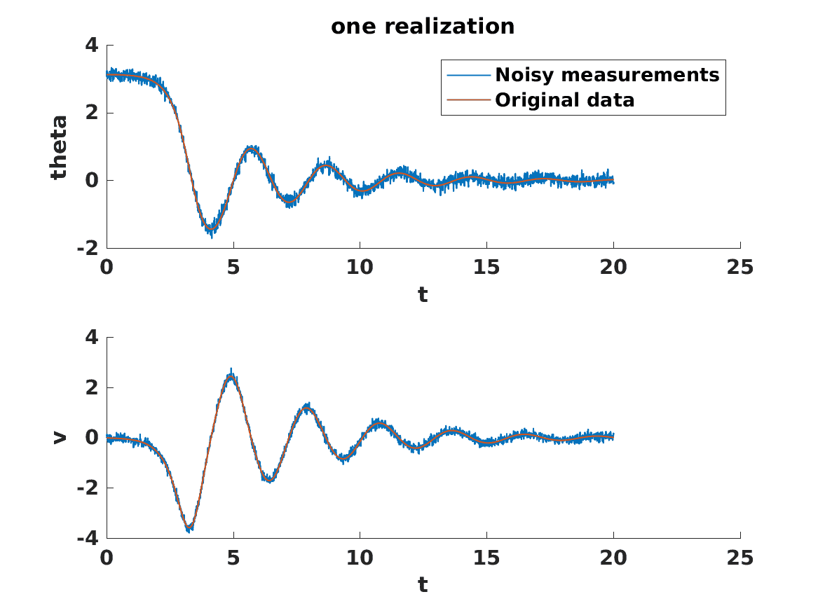
By time $20$ the state has been mostly damped out. We now have everything we need to estimate the length. We run Stan through R. The R script is below and can be found in script.r.
library("rstan")

pendulum_data <- read.csv("pend_noisy.csv")
N <- length(pendulum_data$time) - 1
sigma <- c(0.1,0.1);#velocity, theta std
ts <- pendulum_data$time
ts <- ts[2:length(pendulum_data$time)]
y_init <- c(pendulum_data$velocity[1],pendulum_data$theta[1])
y <- as.matrix(pendulum_data[2:(length(pendulum_data$time)),2:3])
y <- cbind(y[,2],y[,1])
pendulum <- list(N,ts,y_init,y,sigma)


model <- stan_model("pendulum.stan")
fit <- sampling(model, data = pendulum, seed = 123,chains=4,iter=1000, control = list(adapt_delta = 0.99))
print(fit, pars=c("params","z_init"),probs=c(0.1,0.5,0.9),digits=4)
In the terminal, open up R and run
> source("script.r")We now study a couple of cases:
Case 1:
The initial conditions used to generate the measurements and those in the prior are similair. Both the assumed in Stan’s model as well as the matlab script:
$\theta = \pi - 0.01$
$v = 0$
In Stan the conditions have an assumed variance of $0.01^2$ for each parameter. The pendulum length is $1.9$ with variance $0.1^2$ while the true pendulum is of length $2$. The results of the script are
           mean se_mean    sd    10%    50%   90% n_eff   Rhat
params[1] 1.866   0.054 0.076  1.820  1.823 1.998     2 39.819
z_init[1] 0.217   0.302 0.434 -0.038 -0.027 1.049     2 16.054
z_init[2] 1.452   0.527 0.746  1.017  1.023 2.762     2 66.696
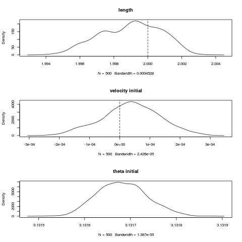
The high Rhat suggests that something is wrong. Debugging Stan code and correctly interpreting the results is a lengthy topic not fully explored here. Further material can be found in the mc-stan forums or in books like “Bayesian Data Analysis Third Edition” by Gelman et. al. We run the following script in R to produce plots in order to further debug:
jpeg('posterior2.jpg')
par(mfrow = c(3,1))
posterior <- extract(fit)
plot(density(posterior$params), main = "length")
abline(v = 2, col = 1, lty = 2)
abline(v =1.867, col = 2, lty = 2)

init = posterior$z_init
init1 = init[,1]
plot(density(init1), main = "velocity initial")
abline(v = 0, col = 1, lty = 2)
abline(v = 0.003, col = 2, lty = 2)

init2 = init[,2]
plot(density(init2), main = "theta initial")
abline(v = 2, col = 1, lty = 2)
abline(v = 3.041593, col = 2, lty = 2)
dev.off()

jpeg('theta2.jpg')
z <- posterior$z
plot(ts,z[1,,1],main="z",xlim=c(0,20),ylim=c(-pi,pi),xlab='Time',ylab='Theta')
for(i in 1:2000){
	print(i)
	par(new=TRUE)
	plot(ts,z[i,,1],add=TRUE,xlim=c(0,20),ylim=c(-pi,pi),xlab='',ylab='')
}
dev.off()
The first plot is the computed by Stan posterior distribution of the length, initial velocity and initial theta. The red is the true initial state specified within the matlab script while black is the computed posterior mean. For both theta and velocity we see a multimodal distribution.
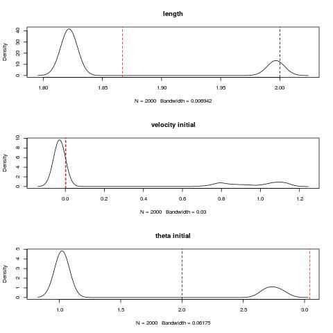
The plot shows that there is no clear guess as to what the initial conditions or the lengths is. The overlay of all the computed simulated $\theta$ s by Stan in the non warm-up phase is below [hence the fat curves].
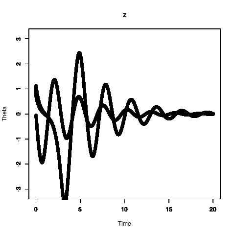
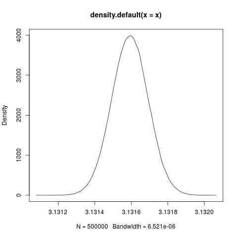
There are two main simulated trajectories of $\theta$. This is because the initial condition and its variance assumed in Stan in variable z_init is too close to $\pi$ as seen in figure below
jpeg('norm.jpg')
x = rnorm(500000,pi-0.01,0.01)
plot(density(x))
abline(v = pi, col = 2, lty = 2)
dev.off()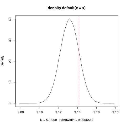
The red line is at $\pi$. Part of the area is over $\pi$ meaning that some conditions are less than $\pi$ while others are greater than. This results in two different types of behaviours of the pendulum swinging down leftwards or rightwards.
Although through the matlab script we technically know the true pendulum length, that knowledge is unknown to the Stan script. If the previous figures in Stan is all that we had to work with then we would have lack confidence in our estimate of the pendulum length.
Case 2:
The variance is now shrunk to avoid having significant probablity for initial $\theta$ greater than $\pi$ to match the actual physical initial conditions defined in matlab script [pendulum falling towards the left]. Variance is now $0.0001^2$ for the prior:
After running Stan again we obtain results that more closely match the true values of the parameters:
           mean se_mean    sd   10%   50%   90% n_eff  Rhat
params[1] 1.999       0 0.002 1.997 1.999 2.001    63 1.000
z_init[1] 0.000       0 0.000 0.000 0.000 0.000   249 0.998
z_init[2] 3.132       0 0.000 3.132 3.132 3.132   154 1.001
In conclusion, this somewhat contrived examples goes to show that knowledge of the priors and model is very important for conducting a successful experiment.