Track the Seals

There is a lot of easily accessible data online waiting to be explored and analyzed. Recently, I came across a work shop for a U.S. Integrated Ocean Observing System (IOOS) Biological Data Training Workshop. Workshops are great as they usually post their code and slide shows for everyone to see and explore. One of the code examples on the posted github dealt with animal telemetry data - let’s explore the data together. First load the libraries

library("rerddap")
library("akima")
library("dplyr")
library("ggplot2")
library("mapdata")
library("ncdf4")
library("plot3D")

ERDDAP is a data server that provides a way to download various scientific data sets. There are lots of various data sets available through IOOS such as trawl surveys, ocean temperatures and others. Coding in R throughout this post, we will first specify the animal telemetry data (gtoppAT):

atnURL <- 'http://oceanview.pfeg.noaa.gov/erddap/'
atnInfo <- info('gtoppAT', url = atnURL)
atnInfo

produces

 Variables:  
     commonName: 
     isDrifter: 
         Range: 0, 1 
     latitude: 
         Range: -77.891, 77.193 
         Units: degrees_north 
     LC: 
     longitude: 
         Range: 0.01, 359.971 
         Units: degrees_east 
     project: 
         Range: 0, 1 
     serialNumber: 
     time: 
         Range: 1.02512583108E9, 1.572152616E9 
         Units: seconds since 1970-01-01T00:00:00Z 
     toppID: 
     yearDeployed: 
         Range: 1995, 9999

which give’s us the data ‘column’ names. Running the command

atnData <- tabledap(atnInfo, fields = c("commonName"), url = atnURL)
atnData

gives us the names of all the animals that are avaiable in the data set:

<ERDDAP tabledap> gtoppAT
   Path: [/home/stan/.cache/R/rerddap/8c470a421cf8d42a59fd20a943fc89dd.csv]
   Last updated: [2019-10-28 17:11:13]
   File size:    [0 mb]
# A tibble: 53 x 1
   commonName            
   <chr>                 
 1 Atlantic Sailfish     
 2 Basking Shark         
 3 Bigeye Tuna           
 4 Black Marlin          
 5 Black-footed Albatross
 6 Blue Marlin           
 7 Blue Shark            
 8 Blue Whale            
 9 California Sea Lion   
10 Common Thresher Shark 
# … with 43 more rows

There are 53 species tracked in the database. Let’s track the one with the largest toppID count

res <- tabledap(atnInfo, fields = c("toppID"), 'commonName="Atlantic Sailfish"', url = atnURL)
maxLength <- length(res$toppID)
maxName <- "Atlantic Sailfish"
for (name in atnData$commonName) {
  cond<-paste('commonName="',name,'"',sep="")
  res <- tabledap(atnInfo, fields = c("toppID"), cond, url = atnURL)

  if(maxLength < length(res$toppID)){
	maxLength = length(res$toppID)
	maxName = name
   }
}
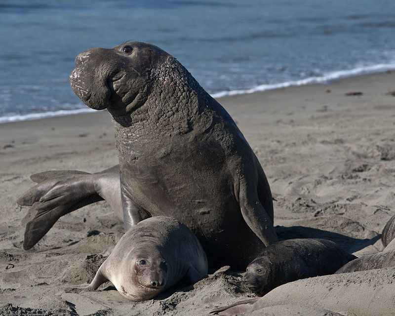
print(paste(maxName,"has the maximum toppID count of",maxLength))

returns

[1] "Northern Elephant Seal has the maximum toppID count of 387"

Here’s a picture of the North Elephant Seal from Wikipedia:

There are a total of 146,668 data entries for the Northern Elephant Seal. Let’s focus on toppID=2006008:

res <- tabledap(atnInfo, fields = c("time","longitude", "latitude","toppID"), 'commonName="Northern Elephant Seal"','toppID="2006008"', orderby="time",url = atnURL)
res$longitude <- as.numeric(res$longitude)
res$latitude <- as.numeric(res$latitude)
xmin<-min(res$longitude-360)
xmax<-max(res$longitude-360)
ymin<-min(res$latitude)
ymax<-max(res$latitude)

w <- map_data("worldHires", ylim = c(ymin,ymax), xlim = c(xmin,xmax))
for
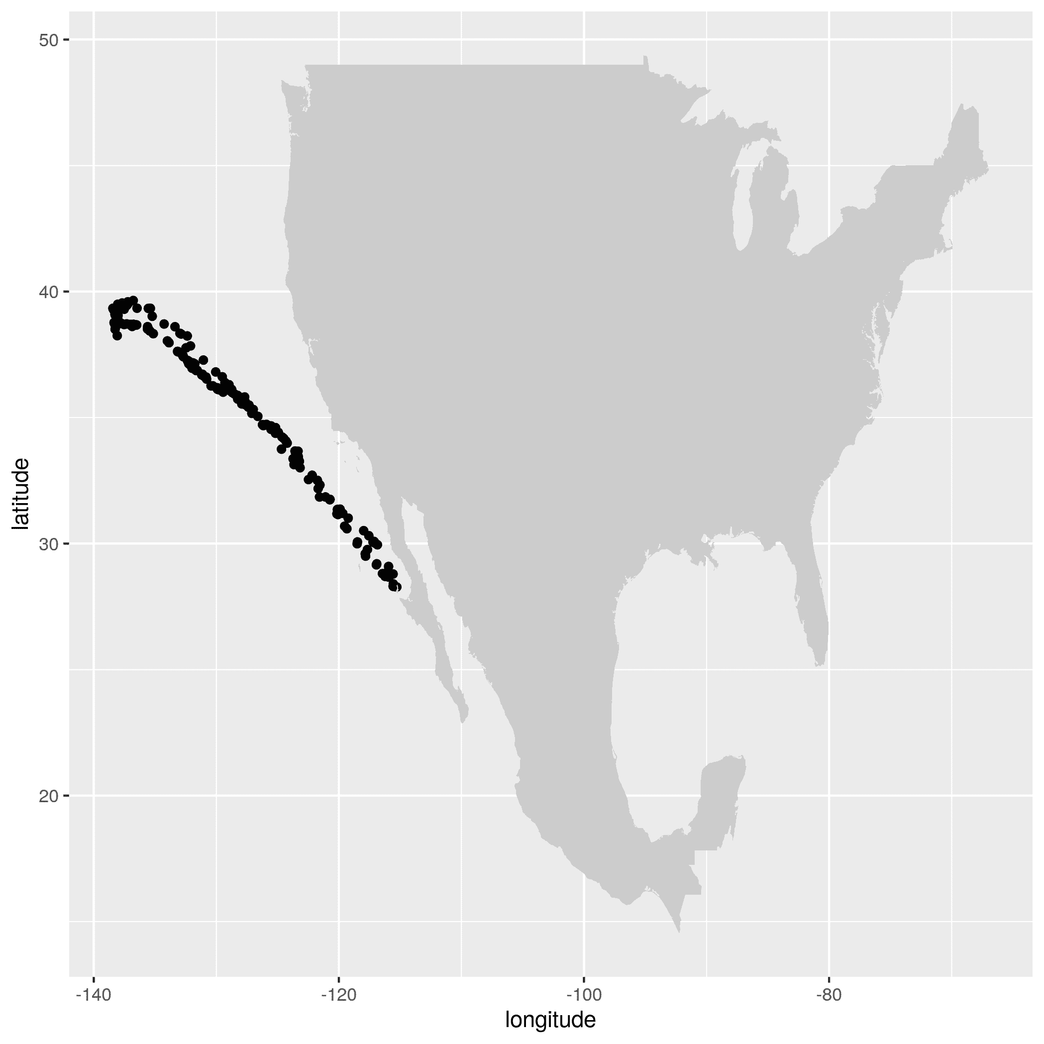
alldata <- data.frame(longitude = res$longitude-360, latitude = res$latitude)
ggplot() + geom_point(data=alldata,aes(x=longitude,y=latitude)) + geom_polygon(data = w,aes(x=long,y=lat,group=group),fill="grey80")

This produces the figure that shows where a specific seal visisted during the time period 2006-01-17 to 2006-05-16:

Let’s animate the results

for (i in 1:length(res$time)){

	alldata <- data.frame(longitude = res$longitude[1:i]-360, latitude = res$latitude[1:i])

	plot = ggplot() + geom_point(data=alldata,aes(x=longitude,y=latitude)) + geom_polygon(data = w,aes(x=long,y=lat,group=group),fill="grey80") + ggtitle(substring(res$time[i],1,10))
	png()
	
	ggsave(plot,file=paste0(i,'.png',sep=""))
	dev.off()
}

in bash run

convert -delay 10 -loop 0 *.png total.gif

to produce