A little bit of SLAM

Let’s work with SLAM. A great series of papers on the topic are here:

Simultaneous Localisation and Mapping (SLAM):Part I The Essential Algorithms - Tim Bailey and Hugh Durrant-Whyte
Simultaneous Localisation and Mapping (SLAM):Part II State of the Art - Tim Bailey and Hugh Durrant-Whyte

Simultaneous Localization and Mapping (SLAM) “problem asks if it is possible for a mobile robot to be placed at an unknown location in an unknown environment and for the robot to incrementally build a consistent map of this environment while simultaneously determining its location within this map.”

Let’s get our hands dirty right away and formulate a system to work with. We will be working with a 2D system where our robot along with landmarks will be treated as (x,y) points. To keep things simple, our robot will be moving on a predefined path such that it does not collide with the landmarks to avoid adding additional logic to the robot. We will be working with Octave.

We first define the robot starting conditions as well as the landmarks:

clear all;
close all;
%set the seed - one of the few commands used here that is _unique_ to Octave
randn("seed",1);

%robot starting initial conditions
robotX = 100;
robotY = 1;

spreadFromCenter=40;
xMin = 100-spreadFromCenter;
xMax=100+spreadFromCenter;
yMin=100-spreadFromCenter;
yMax=100+spreadFromCenter;

%landmarks on the map
xCoords = [80,90,110,120,80,90,110,120];
yCoords = [80,90,110,120,90,100,120,130];
pointNumber = length(xCoords);

Let’s setup the robot’s movement, before worrying about the landmarks. Assume the robot is on a rail road - the y coordinate is unaffected. The robot will be moving at a constant speed with white noise affecting the motion. The following image will describe the situation:

h = figure;
hold on;
scatter(xCoords,yCoords,'*b');
scatter(robotX,robotY,'or','filled');
plot([robotX,robotX],[robotY,200],'k--')
legend('Landmarks','Robot','Robot path');
xlim([100-spreadFromCenter,100+spreadFromCenter]);
ylim([0,200]);
xlabel('x');
ylabel('y');
axis("equal")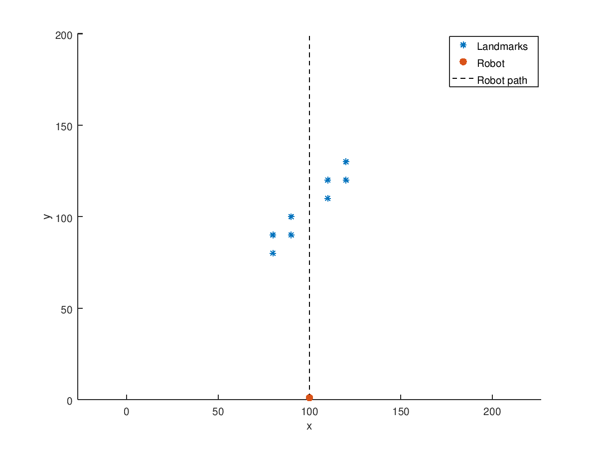

Now lets generate an actual instance of the robot’s motion.

%total timesteps of robot
timesteps = 400;
%speed of the robot (distance covered by timestep)
speed = 0.5;
%function representing the movement - first entry is x coordinate, second y.
next_func= @(coord,time) coord + [0;speed]; 
%process noise - a little noise is added to model in order to be able to do Cholesky decomposition
processNoiseCovariance = [0.00000000001,0;0,0.2];
%store the results
movementCoords = zeros(2,timesteps+1);
%initial conditions
movementCoords(1,1) = robotX;
movementCoords(2,1) = robotY;
for i=1:timesteps
	movementCoords(:,i+1) = next_func(movementCoords(:,i),i) + chol(processNoiseCovariance)'*randn(2,1); 
end

Now, let’s plot the y-coordinate evolution:

h = figure;
plot(1:(timesteps+1),movementCoords(2,:))
ylabel('Y')
xlabel('Time')
axis("equal")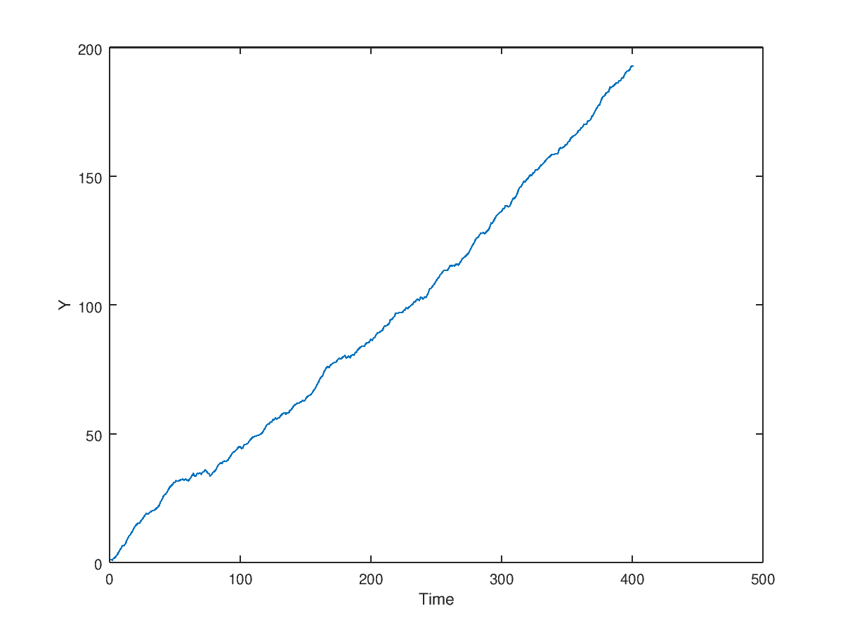

We will set it so that the robot has a maximum measurement radius. Read this for more info on the measurement function used. We will generate noisy measurements of the landmarks based on the position of the landmark.

measurementRadius = 40;
angles = -1*ones(timesteps,pointNumber);
distances = -1*ones(timesteps,pointNumber); 
for i=1:timesteps
	curRobotX = movementCoords(1,i);
	curRobotY = movementCoords(2,i);	

	for j=1:pointNumber
		distance = norm([curRobotX;curRobotY] - [xCoords(j); yCoords(j)]); 
		if distance <= measurementRadius
			distances(i,j) = distance;  
			angles(i,j) = atan2( yCoords(j) - curRobotY , xCoords(j) - curRobotX);
		end	
	end
end
%add noise
angleCovariance = 0.004;
distanceCovariance = 0.2;
anglesNoisy = angles + randn(size(angles)).*sqrt(angleCovariance);
distancesNoisy = distances + randn(size(distances)).*sqrt(distanceCovariance);

Now that we have measurements we are ready to code up our robot exploring the environment. We will assume that the robot does not know now anything about the landmarks:

landMarkDiscoveredCount = 0;

We will set the following variable to be used in identifying if a measurement is associated with a new landmark. If we already are aware that there are n landmarks then we can compare the current measurement’s distance from the estimated location of the other n landmarks to decide if the new measurement is far enough to belong to a new landmark.

minMahalanobisDistance = 7;

The rest of the script is given below. In it the robot moves forward and once it is at the appropriate measurement range, it ‘receives’ measurements from the landmark (the distance and angle with respect to the robot). The robot then decides if it is associated with a new landmark or not. If yes, then it is registered and a new estimate and associated covariance is set up for the landmark’s Kalman filter. Otherwise, the Kalman filter (specifically the update phase) is used to update the estimate (that is closest to the measured landmark).

%estimate location of discovered landmarks
landMarkMeans = {};
%estimate of angle and distance from robot to landmark
landMarkAngleDistances = {};
%associated covariance with landMarkAngleDIstances
landMarkCovariances = {};
%record of measurements 
landMarkMeasurements = {};
%record of all estimates
landMarkEstimates = {};


%creating animation to store images 
%can be a little slow in octave - remove saveas part 
%to just view it
h = figure;
hold on;
axis('equal');
xlim([100-spreadFromCenter,100+spreadFromCenter]);
ylim([0,200]);

for i=1:timesteps
	%current position of robot - here it is known 
	%next extension would let the position be unknown 
	%and the predict phase of the Kalman filter to deal with it
	curRobotX = movementCoords(1,i);
	curRobotY = movementCoords(2,i);	
	
	%there are a total pointNumber landmarks - which our robot has no idea.
	%However, we still have to cycle through all the landmarks at a given timestep
	%in order to simulate an incoming measurement based on measurementRadius value.
	for j=1:pointNumber
		if distances(i,j) ~= -1%-1 flag used to signify that landmark is not in range
			%landmark in measurementRadius range
			%convert the measured angle and distance to an X and Y position
			landmarkX = curRobotX + distancesNoisy(i,j)*cos(anglesNoisy(i,j)); 
			landmarkY = curRobotY + distancesNoisy(i,j)*sin(anglesNoisy(i,j));

			%variables to figure if landmark is new and if not then to 
			%which recorded one does it associate with
			landMarkIndex = 0;
			isNew = false;
			
			%compute distance between measured landmark and all other estimates
			minIndex = 1;
			minVal = -1; 
			for k=1:landMarkDiscoveredCount
				mahalanobisDistance = sqrt( ([landmarkX;landmarkY] - landMarkMeans{k})'
					*([landmarkX;landmarkY] - landMarkMeans{k}));
				if minVal == -1
					minVal = mahalanobisDistance;
				elseif minVal > mahalanobisDistance
					minVal = mahalanobisDistance;
					minIndex = k;
				end
			end
	
			
			if minVal == -1 || minVal > minMahalanobisDistance
				%-1 for first index
				%minVal > ... means that it is far away from all previous measurements
				isNew = true;
				landMarkDiscoveredCount = landMarkDiscoveredCount + 1;
				landMarkIndex = landMarkDiscoveredCount; 
			else
				%measurement is associated with estimate that already exists 
				landMarkIndex = minIndex;
			end

			if isNew ~= true
				%run Kalman filter's update phase 
				
				%to define current estimate we need to compute the angle and distance keeping 
				%in mind that the robot has moved since we computed the estimate last (we are updating
				%the estimate before running the update phase) 
				previous_position = landMarkMeans{landMarkIndex};
				C_measurement = [norm([curRobotX;curRobotY] - [previous_position(1); previous_position(2)]);
					atan2(previous_position(2) - curRobotY,previous_position(1) - curRobotX)];
				%our update phase deals in [distance;angle] format
				%which is converted in the previous calculation meaning
				%that we can set jacobian to the identity matrix
				C_jacobian = eye(2);
				

				%run the update phase
				[estimate_next, covariance_sqrt] = ddekf_update_phase(...
					chol([50*distanceCovariance,0;0,angleCovariance])',...
					chol(landMarkCovariances{landMarkIndex})',...
					C_jacobian,C_measurement,C_measurement,...
					[distancesNoisy(i,j);anglesNoisy(i,j)]);
					
				%store computed results
				landMarkAngleDistances{landMarkIndex} = estimate_next;
				landMarkCovariances{landMarkIndex} = covariance_sqrt*covariance_sqrt';
				landMarkMeans{landMarkIndex} = [curRobotX + estimate_next(1)*cos(estimate_next(2));...
					curRobotY + estimate_next(1)*sin(estimate_next(2))];
				landMarkMeasurements{landMarkIndex}(1:2,end+1) = [landmarkX;landmarkY];
				landMarkEstimates{landMarkIndex}(1:2,end+1) = [landMarkMeans{landMarkIndex}];
			else
				%in case landmark is new, then record results and intialise estimate and covariance 
				landMarkMeans{landMarkIndex} = [landmarkX;landmarkY];
				landMarkAngleDistances{landMarkIndex} = [distancesNoisy(i,j);anglesNoisy(i,j)]; 
				landMarkCovariances{landMarkIndex} = [2*distanceCovariance,0;0,angleCovariance*100];
				landMarkIndex = landMarkDiscoveredCount;
				landMarkMeasurements{landMarkIndex} =  [landmarkX;landmarkY];
				landMarkEstimates{landMarkIndex} = [landMarkMeans{landMarkIndex}];	
			end
		end
	end
	%plot results
	for jj=1:landMarkDiscoveredCount
		for kk=1:length(landMarkMeasurements)
			ttmp = landMarkMeasurements{kk};
			scatter(ttmp(1,end),ttmp(2,end),'r','.')
		end
	end
	%scatter(xCoords,yCoords,'b','*'); %actual location of the landmarks
	f1 = drawCircle(curRobotX,curRobotY,measurementRadius,'g');
	f2 = scatter(curRobotX,curRobotY,'r','filled');
	f3 = plot([curRobotX,curRobotX],[curRobotY,200],'k--');
	
	tmpPlot = [];
	for jj=1:landMarkDiscoveredCount
		ttmp = landMarkMeans{jj};
		tmpPlot = [tmpPlot,scatter(ttmp(1),ttmp(2),"k")];
	end
	%%%REMOVE saveas line for speedup
	saveas(h,strcat('output',num2str(i,'%04d')),'png');
	delete(f1);
	delete(f2);
	delete(f3);
	for jj=1:length(tmpPlot)
		delete(tmpPlot(jj));
	end
	
	pause(0.001)
end

Gif below shows the robot discovering the landmarks. Black circles are the computed estimates while the red dots are the measurements of the landmarks.

How close were the estimates? The blue stars are the true landmark locations, red dots are measurements throughout and black circles are the computed final estimates.

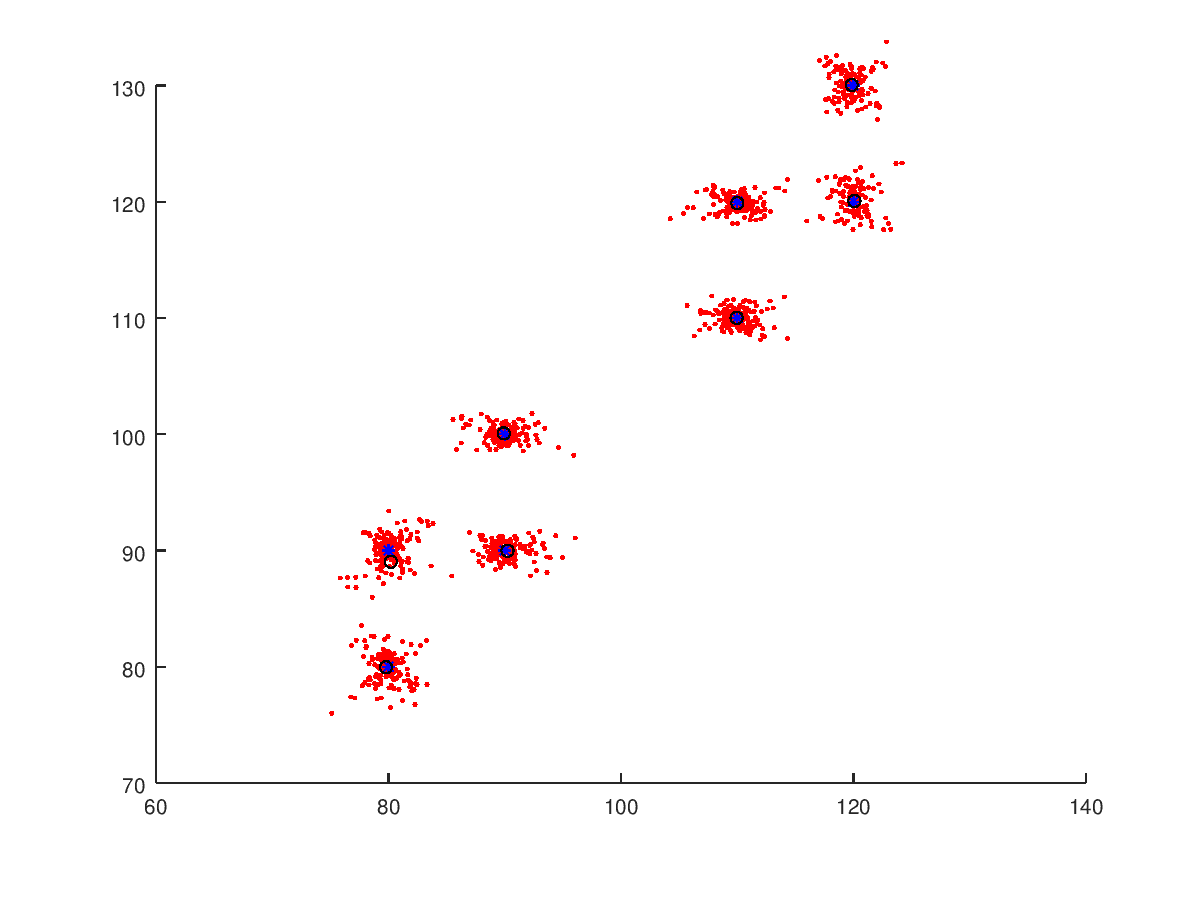
If you want to see the code used here then see script.m and assist file. Also check out this repository that was inspiration for this little project.