TensorFlow Lite Speed Comparison
Hello dear reader!
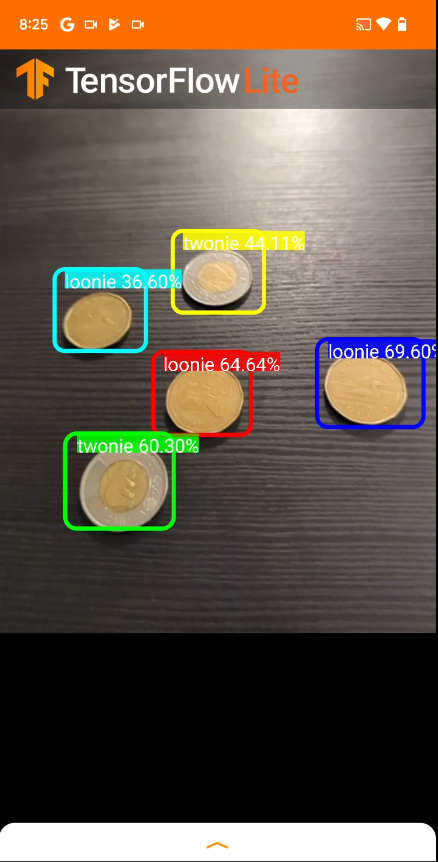
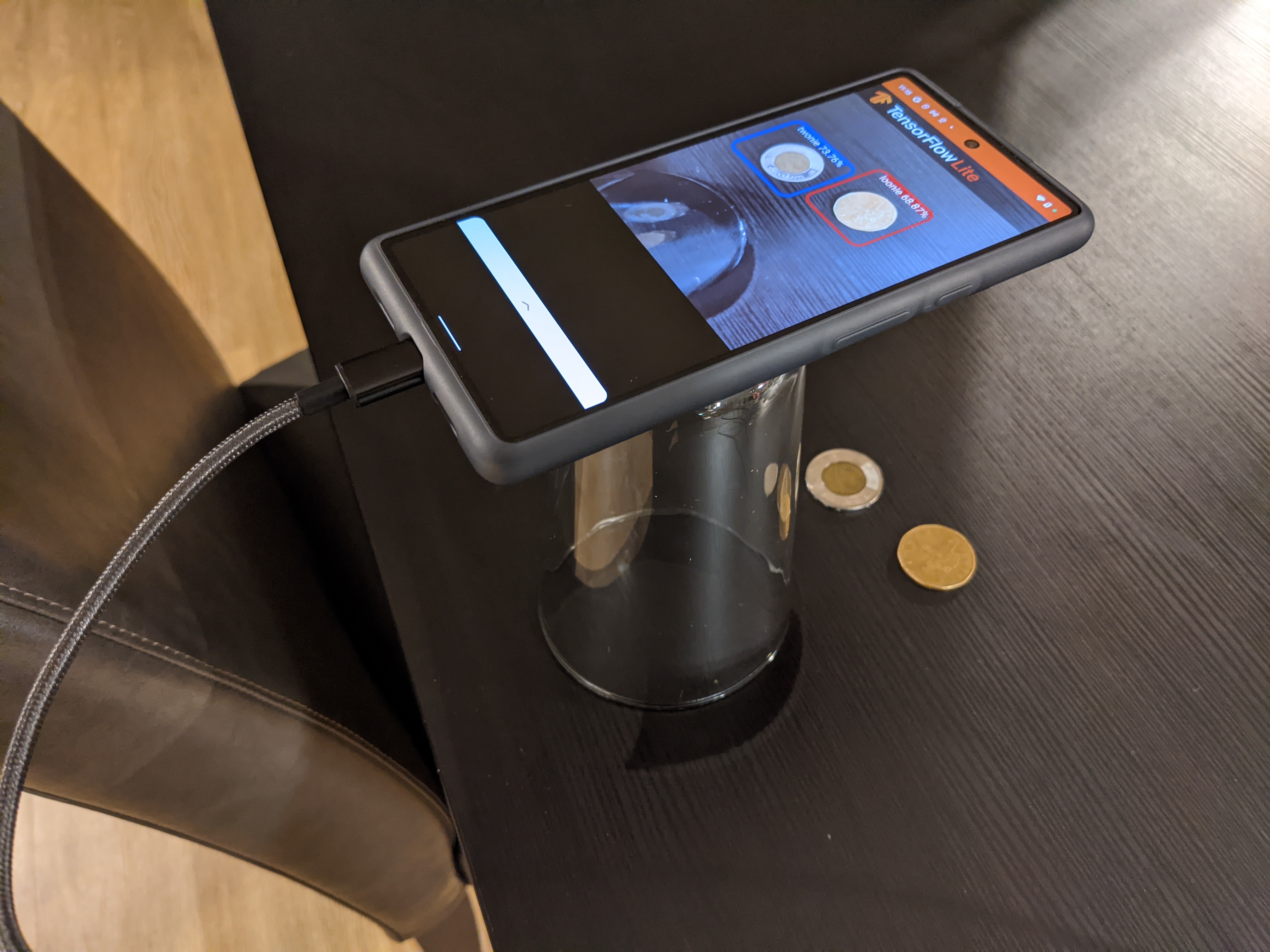
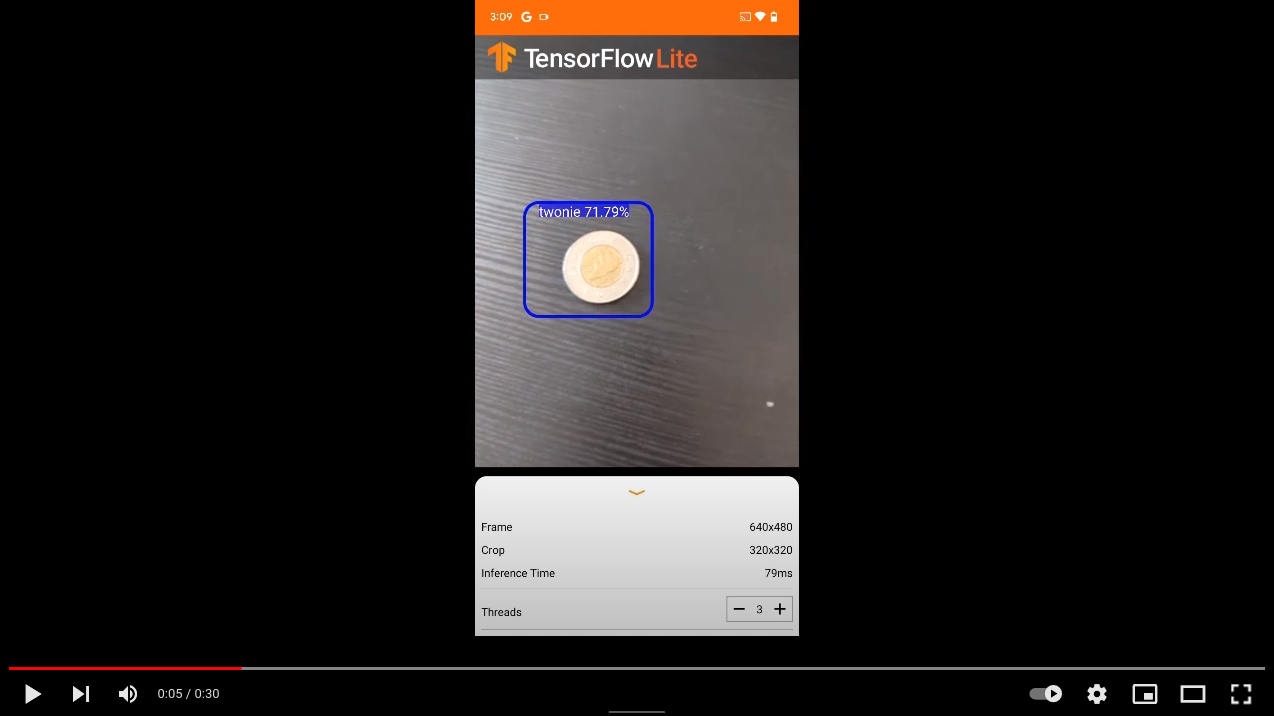
In this blog post we will investigate the speed of TensorFlow Lite models on various Android phones. TensorFlow Lite models are efficient and portable TensorFlow models that are used in machine learning applications on mobile devices like Android phones. In our case we will investigate the models from previous blog post where the models generated can detect coins (see screenshot of app in action below).
We will test two TensorFlow Lite models
-
ssd_mobilenet_v2_fpnlite_320x320_coco17_tpu-8.tar.gzpretrained Tensorflow 2 model which was trained further and converted to Tflite format inresult_2.tflite -
ssd_mobilenet_v3_large_coco_2020_01_14.tar.gzpretrained Tensorflow 1 model which was trained further and converted to Tflite format inresult.tflite
The TensorFlow Lite models are tested on four different Android phones
-
Samsung Galaxy J2 Prime
- 1.5 GB Ram
- 2016 November Release
-
Motorola One Action
- 4 GB Ram
- 2019 October Release
-
Google Pixel 4
- 6 GB Ram
- 2019 October Release
-
Google Pixel 6
- 8 GB Ram
- 2021 October Release
What are we investigating?
We want to test the performance of the TensorFlow Lite models on the various Android phones. When running, the TensorFlow Lite model for input takes an image/snapshot from your cellphone’s camera and processes it and then outputs coordinates of where the detected objects are (in our case these objects are coins). The coordinates are used to plot bounding boxes around the objects as seen in screenshot from cellphone above.
The input output happens over and over again to produce real time object detection. The time to process an image is measured in milliseconds and will be the measure of performance. The speed of processing depends on the TensorFlow model as well as the cellphone’s hardware. The faster the processing time the better the performance.
We will investigate the two TensorFlow Lite models on the four phones to see how they perform. Finally, we want to investigate how to improve performance (i.e. processing time of an image with TensorFlow Lite model) for a fixed phone.
Setup
Here we will briefly discuss the testing procedure used.
The app for benchmark is from tfliteCustomApp repository. To download locally:
git clone https://github.com/mannyray/tfliteCustomApp.git
cd tfliteCustomApp
git checkout benchmark_app
Connect your Android phone to Android Studio and build and then run the app on your phone. result.tflite and result_2.tflite models can be placed in tfliteCustomApp/app/src/main/assets directory by replacing the detect.tflite file.
Make the appropriate modifications (if necessary) to the app in Android Studio and build and run. Usually we are either modifying the exact model used, modifying the thread count or adding a fan to the phone. Your context may vary.
We set the Clear log before launch to enabled in between each run. Run the android app to start logging results.
You can filter for the exact processing times by filter specific log line in Android Studio:
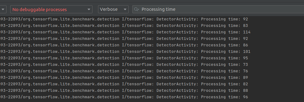
The phone will be connected via USB cable to computer in order to collect logs. The phone will be detecting same objects for duration of your experiment runtime. Once finishing running your app you can copy the logs to a file for later processing.
Results
We will start with looking at a specific cell phone model (Motorola One Action) and look at TensorFlow Lite model performance (the one trained with TensorFlow 1).
We introduce a new parameter, thread count, that can be specified in the app during runtime. We experiment with varying thread count to determine the best performance possible for a given cell phone as the performance varies with thread count. In the figure below we run the app on the phone for thirty seconds. The first 10 seconds are cut off as that is when the application is loading or one is modifying the thread count via UI and so the performance is not stable.
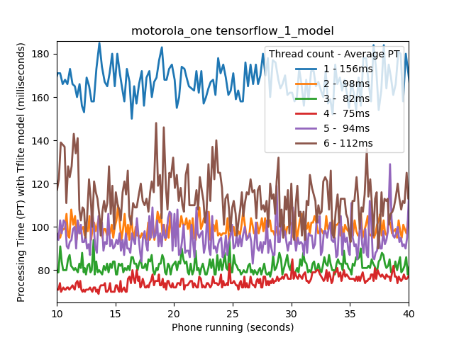
From the figure we can observe that the performance varies significantly when varying thread count. In the case of Motorola One Action running the TensorFlow 2 model, we have the red line, representing four thread count, is the best performing configuration with average processing time of 75ms. When we decrease OR increase thread count from four we increase the processing time. For low and high thread count (1 or 6) we observe the variance in processing time has increased compared to the optimal thread count of four.
The previous image was specifically for Motorola One Action. What happens if we fix a TensorFlow Model and see how the various Android models perform? In the image below we plot the average one minute performance of each of the four cell phones on the TensorFlow 1 trained model while we vary the thread count.
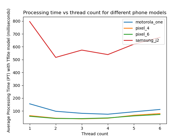
The old Samsung J2 prime is so slow that we cannot really see how well the others are performing. We can tell that the other phones are much better with the Pixels being the best and near each other performance wise. Let us see what happens when we normalize each of the curves in the figure above based on its maximum value (we normalize each curve by dividing each value by the largest value present in the curve which reduces the values to range of zero to one):
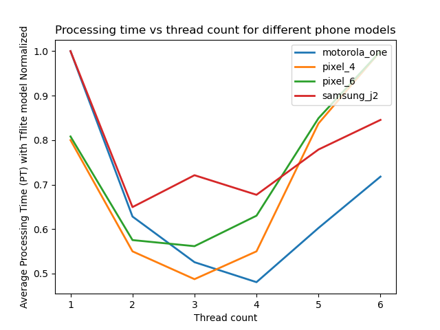
The maximum values are either with one thread count or six as that is where the cell phone is the most slowest. For all the cell phones we can tell that the optimal performance is somewhere in between one and six threads. For Motorola One Action and Pixel 4 we observe that the optimal time is twice as good as the worst processing time (0.5 ratio). We observe that some phones are optimal at three threads while others at four (Pixel 4 vs Motorola One Action).
With the previous figure we lose the ability to compare performance of a cell phone to another cell phone. Let us compare the fastest processing time (among all thread counts) for all cell phones against each model. The processing time is the average of one minute.
| TensorFlow 1 Model | TensorFlow 2 Model | |
|---|---|---|
| Samsung J2 Prime | 517ms | 1174ms |
| Motorola One Action | 75ms | 216ms |
| Pixel 4 | 39ms | 102ms |
| Pixel 6 | 41ms | 82ms |
We observe that the TensorFlow 2 model is slower for all the cell phones by at least a factor of two. We observe that Pixel 6 is the fastest but comparable to Pixel 4 when using TensorFlow 1 model ( 39ms to 41ms too close say one is better than the other).
It is important to note that I do not mean that TensorFlow 1 is better than TensorFlow 2. When I use “TensorFlow N model” I am referring to with which version the model was trained with. The models themselves are different which you can confirm yourself by analyzing the .tflites in https://netron.app/. Due to TensorFlow versioning and based on the work here each model can only be created in that specific version of TensorFlow. The TensorFlow 1 model is more lightweight so it is expected that it performs better. Lightweight models can be found in TensorFlow 2 as well.
When using some other model for your application you will have to consider its speed and understand that it can have a significant impact on performance as demonstrated in the table above. You will also have to to consider its ability of correctly detecting objects. I happened to train these specific models as these were the first ones I was able to setup the training data to TensorFlow Lite model pipeline successfully. TensorFlow pipeline can be a pain to setup.
In addition, you will also have to consider the phone model. In our study the Samsung J2 Prime was the slowest phone and not competitive to others. What if we compare the Motorola One Action and Pixel 4 for the TensorFlow 1 Model. The former is 75ms while the latter is 39ms in average processing time. Is 75ms sufficient for your specific application?
Let us assume your application is for tracking an object as it moves across a screen as it was in my application. For the purpose of tracking I implemented a Simple Online Realtime Tracking algorithm which is built on top of a Kalman Filter. In tracking applications, we need to make sure we have an accurate estimate of where our object is located. Our estimate of where the object is located depends on how frequently we obtain our measurements (among other things). For TensorFlow Lite models, the measurements are the bounding boxes around detected objects. In the video below observe the difference in lag of the bounding box as the thread count is increased and thus processing time.
An extreme example of tracking lag is if you are tracking an ant on the ground but you can only check once a minute. Last time you saw the ant, he was heading north. In a minute you expect him to be slightly north of where you last saw him. What if the ant turned west half way through the one minute? Now you have to search the ground for the ant. If you were checking once every 10 seconds you wouldn’t have to spend as much time looking for him even if he changed direction. Frequency of measurements is relevant to your ability to track. If we double the processing time from one phone model to the next (or from one TensorFlow model to the next) then this can have significant impact on you as your measurements are less frequent.
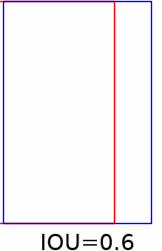
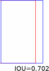
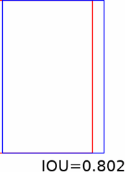
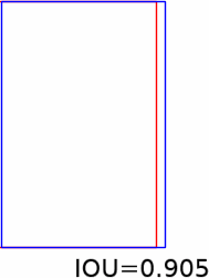
In tracking, a cost function of accuracy is the Intersection Over Union measure. In the gif below consider the red is the true position of an object and blue box where you think it is. As the blue box more closely matches the location of the red, the IOU increases to a maximum of one. IOU is zero when there is no intersection.

Some stills from the gif above:
 |
 |
 |
 |
In the image below I plot the IOU as I increase the time difference between arriving measurements in a simulation I ran here (see example 13). The increase in time between arriving measurements could represent increased processing time for TensorFlow model. Too much lag can significantly reduce IOU (see black line and red line). The stills from gif can help get an idea of significance of lower IOU.
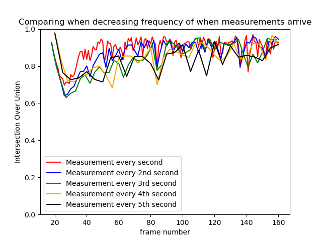
You can always tune the Kalman filter or Simple Online Realtime Tracking algorithm to account for slower processing time but it can be annoying especially if you are not familiar with the algorithm. The faster the TensorFlow model the less you need to rely on your Kalman filter. For examples on tuning please see my work here.
So far we have investigated processing time over a small period of time of thirty seconds. For tracking applications (or others) you may want to run your app for much longer. Let us see what happens when we increase runtime to fifteen minutes.
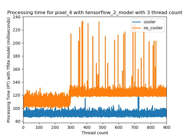
In this case we are running the Pixel 4 with TensorFlow 2 model. The blue line is us running with a cooling fan while the orange is just the phone on its own. Images of the fan are below. It attaches to the phone directly.
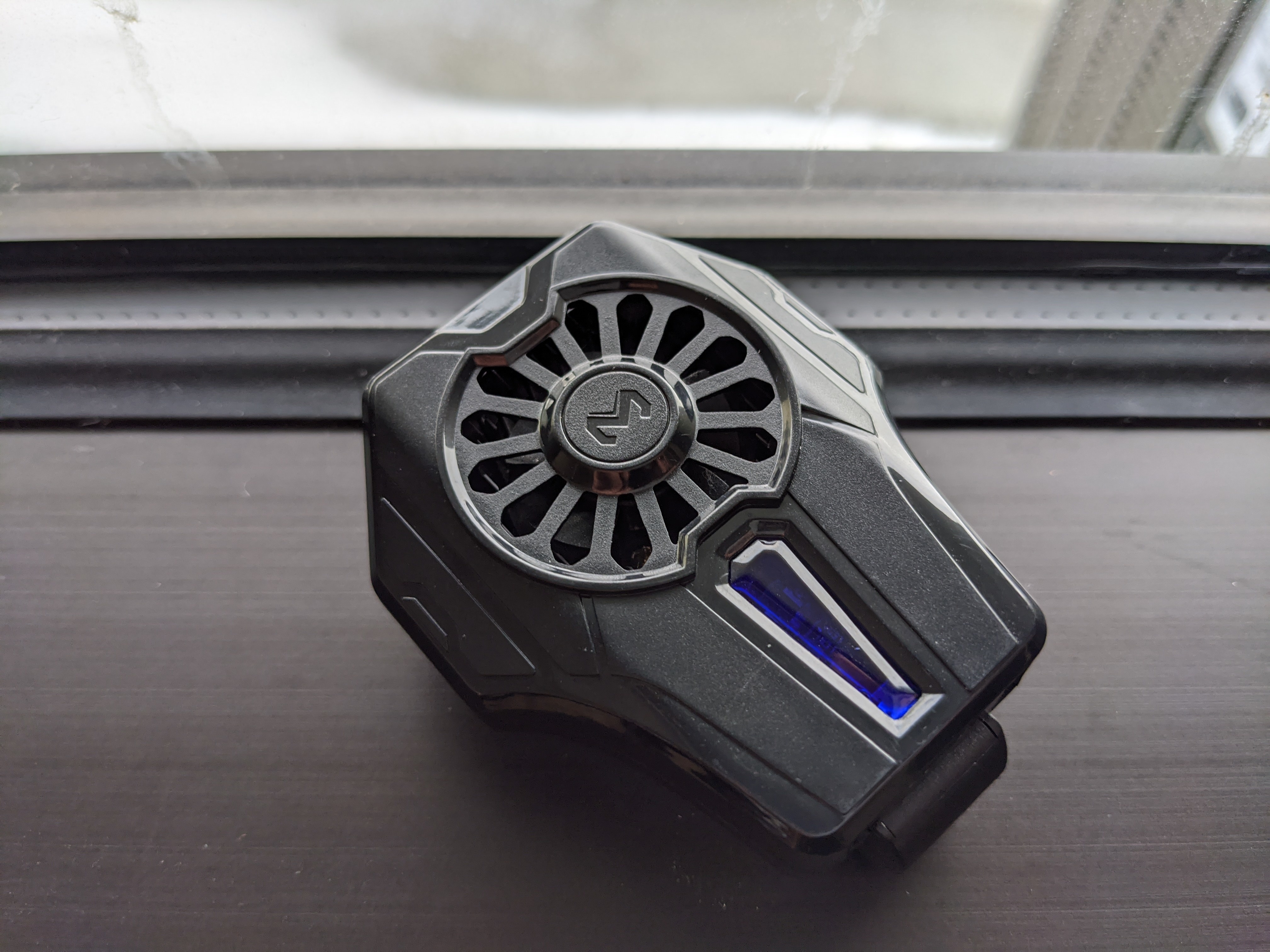 |
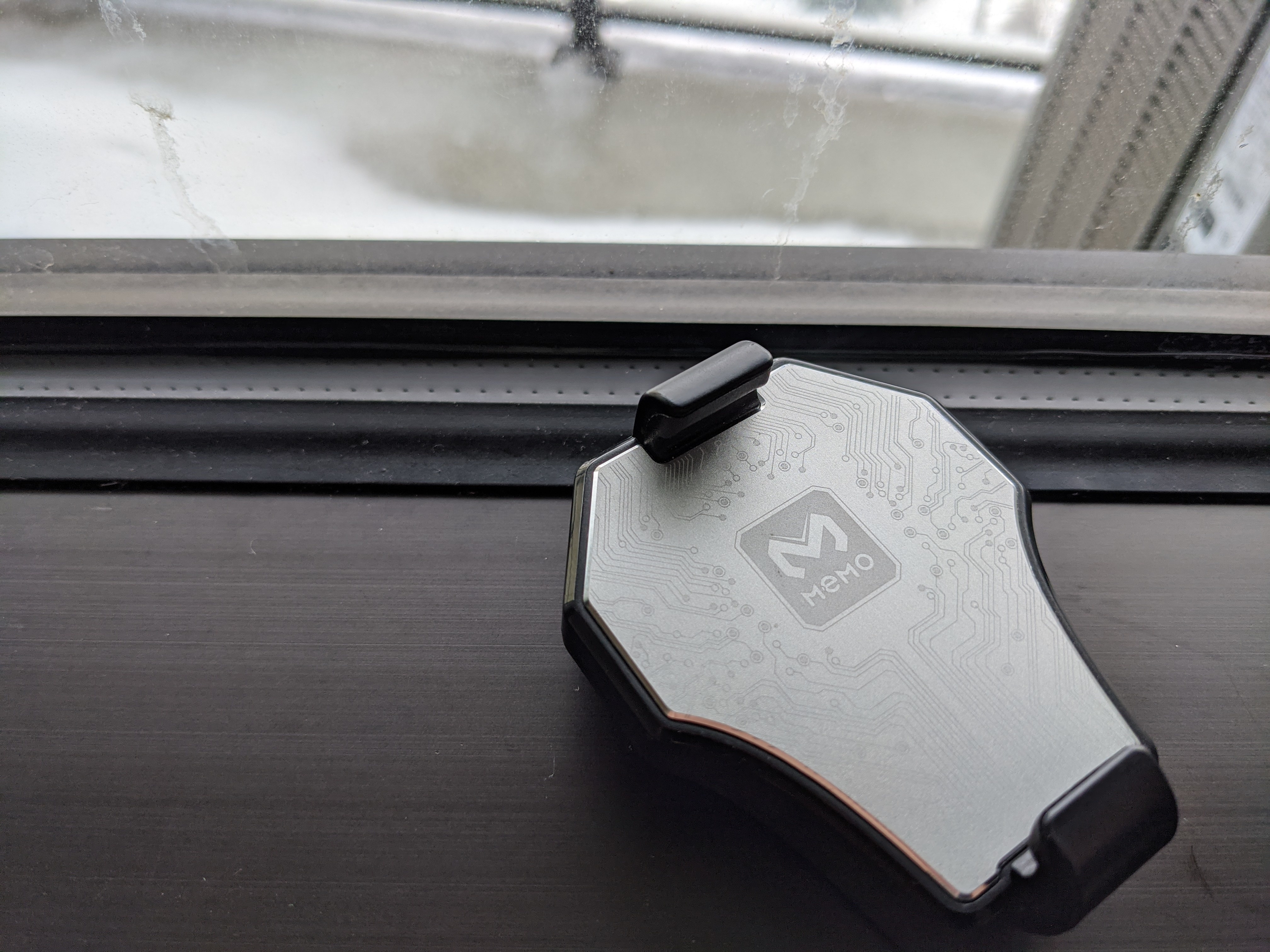 |
With the fan, the average processing time is around 90ms while without the average is at first 110ms and then increases to around 130ms. Without the fan, the phone gets really hot and overtime can shutdown from overheating.
Adding a fan is one quick way to improve your application’s performance in the long run.
Conclusion
In this blog post I analysed the performance of TensorFlow Lite models on various Android phones and provided real world numbers. I briefly discussed TensorFlow Lite models in the context of object tracking applications. Finally, I provided a good tip for long term TensorFlow Lite execution on the phone: using a fan.
The applications of TensorFlow Lite models seem endless to me. I am very grateful that TensorFlow has provided the technology for developing these models and has provided sample code for which I can easily get started in creating these applications like in the case of the benchmark app. A recent application in which I used some of the information presented here can be found in a previous post about a prototype. The gif of the prototype, that tracks oranges, is below. I hope the reader finds the information presented here useful for their experiments too.